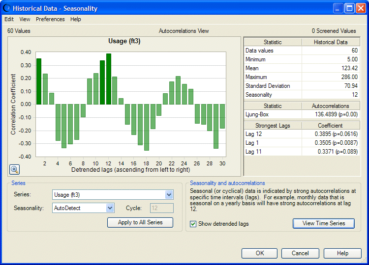
The Autocorrelations view of the Historical Data dialog displays a chart of autocorrelations— correlations of values of the same series separated by varying time lags—to indicate whether the historical data values have seasonality (Figure 3, Historical Data – Seasonality Dialog — Autocorrelations View).
Note: | Viewing Historical Data by Seasonality describes the Historical Data - Seasonality dialog. |
Other dialog features:
In Autocorrelations View, the series chart plots autocorrelation coefficients at different lags for the selected series (three greatest lags are plotted with darker bars); seasonality is indicated by strong lags at certain time periods.
To show or remove trend corrections from the chart and statistics tables, select or clear Show detrended lags . For more information about lags and the Ljung-Box statistic, see Notes about Autocorrelations.
To enlarge the chart, click + in the lower-left corner and move the sliders to show different levels of detail.
To view seasonality in terms of historical data values for each series, click View Time Series. The seasonality chart changes to Chart View, a plot of historical data values over time. For more information, see Viewing Historical Data by Seasonality.
If you selected more than one historical data series, change the graph to view another data series by selecting it from the Series list.
The lag represents the number of data periods that the data is offset with the original data before calculating the correlation coefficient. For example, a lag of 12 corresponds with correlating the data with itself, offset by 12 periods; in other words, the correlation of the first data item with the thirteenth data item, the second data item with the fourteenth data item, and so on. The p-value (value of Prob) in the statistics table indicates the significance of the lag and is detrended or not, depending on the check box selection in Autocorrelations View.
A seasonal series has alternating patterns of positive and negative lags. The seasonality (cycle) is usually determined by the strongest lag in the set of positive lags following the first set of negative lags.
Seasonality is always calculated on detrended lags to remove the effect that trending data has on autocorrelations. You can select or clear Show detrended lags to view autocorrelation information with or without detrending.
If the probability of the Ljung-Box statistic is less than 0.05, the set of autocorrelations is significant, and the data is probably seasonal. The seasonality is indicated by the autocorrelation lag. For example, if one of the top three lags is 12 and has a probability of less than 0.001, the data probably have a seasonality of 12 periods.
