Engineering Modeling

Correlation of Duke Basketball Scores, in ModelRisk (7/8)

Karl - CB Expert

Share:

Print

Rate article:

No rating
Rate this article:
No rating

Correlation behavior in ModelRisk is enforced with the use of copulas. Copulas offer more flexibility in accurately simulating real data scatter-plot patterns than do single-value correlation coefficients. While this advantage is clear for financial and insurance applications, its implementation in an MCA spreadsheet simulator can make the difference between universal adoption and rejection by a majority of the intended user group. Let us now use ModelRisk (MR) to enforce the correlation behavior between Duke Basketball offense scores and their opponents' scores, based on the '09/'10 historical data.

Much like MR's distribution-fitting capability, MR's copula-fitting capability can create MR Objects that represent the copulas. It is accessed through the same "Fit" command. As will be seen with the first drop-down menu, copulas can be created between either paired data sets (bivariate) or more than two sets of data (multivariate). With ModelRisk up and running within MS Excel, open the latest version of the Duke 09_10 Scores file. It does not matter what the active cell is when performing this operation:

  • Select "Fit" in MR ribbon bar.
  • Select "Bivariate Fit Copula" from drop-down menu.
  • Select all the potential copulas from the list on left-hand side. (Use CTL-CLICK to select multiple copulas.)
  • Select right-arrow button to place selected copulas into list on right-hand side.
  • Select "OK."
  • Using cell-reference-picker in "Source data" box in upper left-hand corner, identify Cells C4:D37 as the source data.

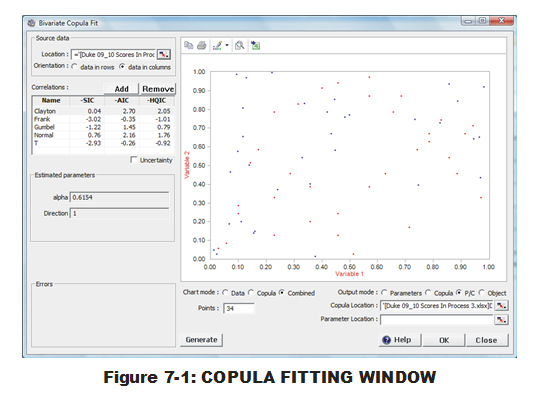
At this point, the user will be presented (Fig. 7-1) with scatter plot of both the data (red) and points representing sampled data produced with this copula (blue). (This can be manipulated to show only the data or the copula via radio buttons below.) A list of copulas appears beneath "Correlations:" (below the 'Source data' box in upper left-hand corner). Note that the same three criteria used in MR distribution-fitting are being employed here. Careful examination of the criteria values for all five Copulas are not consistent down the board so the user is recommended to click once on the top of each criteria column to understand how the criteria are in disagreement about the fitting order. It appears, however, that all three agree on the top two (Normal & Clayton) while the lower three remain in the same order.

The user decision of which copula to employ is fraught with more black magic than with selecting distributions. What are the significant differences between Normal and Clayton that would move a user to choose one over the other? For these bivariate copulas, it may not make a difference. If the basketball SME examined the scatter plot and deduced that positive correlation behavior was stronger at one end of the scoring scale (for both teams) than the other, the Archimedean Clayton would be more appropriate than Normal since it can reproduce that type of localized correlation. But this judgment is difficult to do with 34 samples. (Perhaps it could be justified if other teams have much better copula fits to Clayton than Normal?) For the current data set, we will use Bivariate Clayton since it was selected as best by two out of three criteria. We should still be uncertain about its suitability over Normal and question that assumption when more data arrives.

We will now use an option above the scatter plot to insert a MR Object into the spreadsheet. (This could also be done via options in the lower right-hand corner. However, it appears this is a remnant of an older feature, before MR Objects were implemented. By using the options in lower right-hand corner, the user must select the "OK" button for the appropriate MR entities to be placed into the spreadsheet. Unfortunately, that closes the Bivariate Copula Fit window when the user might want to do more in that window. The approach defined here allows the window to stay open after the operation is completed.)

  • Select "Clayton" in the list of copulas beneath "Correlations:"
  • Select the 'Excel-with-plus-sign' icon above displayed scatter plot.
  • Select "Object" from drop-down menu.
  • Select Cell U25.
  • Select "OK." (These steps place the MR Object into the designated cell.)
  • Select "OK" to exit the Bivariate Copula Fit window.

The MR Object for the Bivariate Clayton, as fit to the data, now resides in Cell U25. Just like with the MR Objects for distributions, we must add a few more details to our spreadsheet to connect this copula Object to the simulated values of the two PDFs. That is done by entering information into two cells that, when linked to the copula, will then connect a paired set of simulated values to two PDF Objects via the copula Object.

  • Select Cells P24:P25 via click-and-drag.
  • Enter "=VoseCopulaSimulate(U25)" and hit CTL-SHIFT-ENTER. (It is important to not just hit ENTER to conclude entry. The user is entering an array formula between two cells and must use CTL-SHIFT-ENTER to complete array formula entry properly. If done correctly, the user should see curly bracket around the formula displayed in the formula bar.)
  • Select Cell P5.
  • Modify formula to become "=VoseSimulate(U5, P24)" and hit ENTER.
  • Select Cell P15.
  • Modify formula to become "=VoseSimulate(U15, P25)" and hit ENTER.

The reason for this coupling is driven by how the VoseSimulate function provides sampled values. The first argument in a VoseSimulate function is referring to the MR Object of the distribution to be sampled from. If there is no second argument, VoseSimulate will randomly and without connection to any other distribution or copula, generate values. If there is a second argument, that value is specifying an exact percentile to be produced from the first argument's distribution Object. By specifying the second VoseSimulate arguments to relate back to the paired VoseCopulaSimulate functions in Cells P24:P25, we are forcing correlation into the two VoseSimulate functions.

One might argue that implementation of copulas in MR requires more fore-thought and work on the part of the analyst. Perhaps too much work? Does the user understand enough about copula behavior to use the linked formulas and create the appropriate correlation behavior during simulation? If not, a CB correlation interface (via the "Define Assumption" options), may be the best way to go. Perhaps the flexibility in using copulas is necessary (finance & insurance)? If yes, MR provides this capability while CB does not.

Let us stand back and consider pros and cons of either software for discrete distribution fitting and enforcing correlations in simulations. And the winner is … ?

Comments

Collapse Expand Comments (0)
You don't have permission to post comments.

Oracle Crystal Ball Spreadsheet Functions For Use in Microsoft Excel Models

Oracle Crystal Ball has a complete set of functions that allows a modeler to extract information from both inputs (assumptions) and outputs (forecast). Used the right way, these special Crystal Ball functions can enable a whole new level of analytics that can feed other models (or subcomponents of the major model).

Understanding these is a must for anybody who is looking to use the developer kit.

Why are analytics so important for the virtual organization? Read these quotes.

Jun 26 2013
6
0

Since the mid-1990s academics and business leaders have been striving to focus their businesses on what is profitable and either partnering or outsourcing the rest. I have assembled a long list of quotes that define what a virtual organization is and why it's different than conventional organizations. The point of looking at these quotes is to demonstrate that none of these models or definitions can adequately be achieved without some heavy analytics and integration of both IT (the wire, the boxes and now the cloud's virtual machines) and IS - Information Systems (Applications) with other stakeholder systems and processes. Up till recently it could be argued that these things can and could be done because we had the technology. But the reality is, unless you were an Amazon, e-Bay or Dell, most firms did not necessarily have the money or the know-how to invest in these types of inovations.

With the proliferation of cloud services, we are finding new and cheaper ways to do things that put these strategies in the reach of more managers and smaller organizations. Everything is game... even the phone system can be handled by the cloud. Ok, I digress, Check out the following quotes and imagine being able to pull these off without analytics.

The next posts will treat some of the tools and technologies that are available to make these business strategies viable.

Multi-Dimensional Portfolio Optimization with @RISK

Jun 28 2012
16
0

Many speak of organizational alignment, but how many tell you how to do it? Others present only the financial aspects of portfolio optimization but abstract from how this enables the organization to meets its business objectives.  We are going to present a practical method that enables organizations to quickly build and optimize a portfolio of initiatives based on multiple quantitative and qualitative dimensions: Revenue Potential, Value of Information, Financial & Operational Viability and Strategic Fit. 
                  
This webinar is going to present these approaches and how they can be combined to improve both tactical and strategic decision making. We will also cover how this approach can dramatically improve organizational focus and overall business performance.

We will discuss these topics as well as present practical models and applications using @RISK.

Reducing Project Costs and Risks with Oracle Primavera Risk Analysis

.It is a well-known fact that many projects fail to meet some or all of their objectives because some risks were either: underestimated, not quantified or unaccounted for. It is the objective of every project manager and risk analysis to ensure that the project that is delivered is the one that was expected. With the right know-how and the right tools, this can easily be achieved on projects of almost any size. We are going to present a quick primer on project risk analysis and how it can positively impact the bottom line. We are also going to show you how Primavera Risk Analysis can quickly identify risks and performance drivers that if managed correctly will enable organizations to meet or exceed project delivery expectations.

.


Modeling Time-Series Forecasts with @RISK


Making decisions for the future is becoming harder and harder because of the ever increasing sources and rate of uncertainty that can impact the final outcome of a project or investment. Several tools have proven instrumental in assisting managers and decision makers tackle this: Time Series Forecasting, Judgmental Forecasting and Simulation.  

This webinar is going to present these approaches and how they can be combined to improve both tactical and strategic decision making. We will also cover the role of analytics in the organization and how it has evolved over time to give participants strategies to mobilize analytics talent within the firm.  

We will discuss these topics as well as present practical models and applications using @RISK.

The Need for Speed: A performance comparison of Crystal Ball, ModelRisk, @RISK and Risk Solver


Need for SpeedA detailed comparison of the top Monte-Carlo Simulation Tools for Microsoft Excel

There are very few performance comparisons available when considering the acquisition of an Excel-based Monte Carlo solution. It is with this in mind and a bit of intellectual curiosity that we decided to evaluate Oracle Crystal Ball, Palisade @Risk, Vose ModelRisk and Frontline Risk Solver in terms of speed, accuracy and precision. We ran over 20 individual tests and 64 million trials to prepare comprehensive comparison of the top Monte-Carlo Tools.


Excel Simulation Show-Down Part 3: Correlating Distributions

Escel Simulation Showdown Part 3: Correlating DistributionsModeling in Excel or with any other tool for that matter is defined as the visual and/or mathematical representation of a set of relationships. Correlation is about defining the strength of a relationship. Between a model and correlation analysis, we are able to come much closer in replicating the true behavior and potential outcomes of the problem / question we are analyzing. Correlation is the bread and butter of any serious analyst seeking to analyze risk or gain insight into the future.

Given that correlation has such a big impact on the answers and analysis we are conducting, it therefore makes a lot of sense to cover how to apply correlation in the various simulation tools. Correlation is also a key tenement of time series forecasting…but that is another story.

In this article, we are going to build a simple correlated returns model using our usual suspects (Oracle Crystal Ball, Palisade @RISK , Vose ModelRisk and RiskSolver). The objective of the correlated returns model is to take into account the relationship (correlation) of how the selected asset classes move together. Does asset B go up or down when asset A goes up – and by how much? At the end of the day, correlating variables ensures your model will behave correctly and within the realm of the possible.

Copulas Vs. Correlation

Copulas and Rank Order Correlation are two ways to model and/or explain the dependence between 2 or more variables. Historically used in biology and epidemiology, copulas have gained acceptance and prominence in the financial services sector.

In this article we are going to untangle what correlation and copulas are and how they relate to each other. In order to prepare a summary overview, I had to read painfully dry material… but the results is a practical guide to understanding copulas and when you should consider them. I lay no claim to being a stats expert or mathematician… just a risk analysis professional. So my approach to this will be pragmatic. Tools used for the article and demo models are Oracle Crystal Ball 11.1.2.1. and ModelRisk Industrial 4.0

Excel Simulation Show-Down Part 2: Distribution Fitting


One of the cool things about professional Monte-Carlo Simulation tools is that they offer the ability to fit data. Fitting enables a modeler to condensate large data sets into representative distributions by estimating the parameters and shape of the data as well as suggest which distributions (using these estimated parameters) replicates the data set best.

Fitting data is a delicate and very math intensive process, especially when you get into larger data sets. As usual, the presence of automation has made us drop our guard on the seriousness of the process and the implications of a poorly executed fitting process/decision. The other consequence of automating distribution fitting is that the importance of sound judgment when validating and selecting fit recommendations (using the Goodness-of-fit statistics) is forsaken for blind trust in the results of a fitting tool.

Now that I have given you the caveat emptor regarding fitting, we are going to see how each tools offers the support for modelers to make the right decisions. For this reason, we have created a series of videos showing comparing how each tool is used to fit historical data to a model / spreadsheet. Our focus will be on :

The goal of this comparison is to see how each tool handles this critical modeling feature.  We have not concerned ourselves with the relative precision of fitting engines because that would lead us down a rabbit hole very quickly – particularly when you want to be empirically fair.

RESEARCH ARTICLES | RISK + CRYSTAL BALL + ANALYTICS