In past blogs, I have waxed eloquent about two traditional methods of performing Tolerance Analysis, the Worst Case Analysis and the Root Sum Squares. With the advent of ever-more-powerful processors and the increasing importance engineering organizations place on transfer functions, the next logical step is to use these resources and predict system variation with Monte Carlo Analysis.

The name Monte Carlo is not by accident. This methodology uses the random behavior associated with underlying probability distribution to sample from those PDFs. Thus, it resembles gambling where players predict outcomes on games of random chance. At the time of its "invention," Monte Carlo in Monaco was considered the gambling capitol of the world, thus the name. (Perhaps if it had been "invented" later, it would've been called Las Vegas or Macau?)

The methodology is simple in nature but with a far-reaching impact in the prediction world. In the RSS methodology, the 1^st and 2^nd derivatives of transfer functions have primary influence over system output means and standard deviations (when variation is applied to the inputs). But there are no mathematical approximations to capture system variation in Monte Carlo analysis. 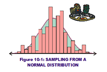Instead, it uses random sampling methods on defined input PDFs and applies those sampled values to the transfer functions. (Figure 10-1 displays a potential sampling from an input's Normal distribution, in histogram format, overlaid on the normal curve itself.) The "math" is much simpler and we let our laptops crunch numbers and predict outcomes.

This sampling is done many times over, usually thousands of times. (Each combination of sampling is considered a trial. All combined trials run constitute one simulation.) Every time a sampling is done from all the input PDFs, those single-point values are applied to the transfer function and the thousands of possible output values are recorded. They are typically displayed as histograms themselves.

Returning to the RSS graphical concepts covered in the last couple of posts, let us examine this approach using an exponential transfer function (see Figure 10-2). We apply a normal PDF to the input (horizontal) axis which is then sampled many times over (many trials 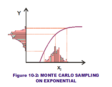displayed as a histogram of sampled values). Applying these numerous sampled values to the exponential curve, the corresponding numerous output values are calculated and then displayed also in histogram format along the output (vertical) axis. These thousands (or millions) of trials allow us to capture the output variations visually, perhaps even approximate their behavior with a PDF that "fits" the data. We can also perform statistical analysis on the output values and predict the quality of our output variations. Perhaps some fall outside the LSL & USL limits? Their probability of occurrence quantifies the quality of the system output. Voila! No need to scratch out 1^st and 2^nd derivatives like in RSS. All methods require transfer functions but with Monte Carlo analysis, thorny calculus falls by the wayside.

Now let us apply this methodology to the one-way clutch example. Thanks for staying tuned!

Hambleton, Lynne, Treasure Chest of Six Sigma Growth Methods, Tools, and Best Practices (2008); Prentice Hall, pp. 431-432.

Sleeper, Andrew D., Six Sigma Distribution Modeling (2006); McGraw-Hill, pp. 115-118.