 With uncertainty and risk lurking around every corner, it is incumbent on us to account for it in our forward business projections, whether those predictions are financially-based or engineering-centric. For the design engineer, he may be expressing dimensional variance in terms of a tolerance around his nominal dimensions. But what does this mean? Does a simple range between upper and lower values accurately describe the variation?
It does not. The lower and upper bounds of a variable say nothing about specific probabilities of occurrence within that range. To put it another way, there is no understanding of where those dimensional values will be more likely to occur within that range. That can have far-reaching consequences when trying to control the variation of a critical output. Therefore, world-class quality organizations capture variable behavior with probability distributions.
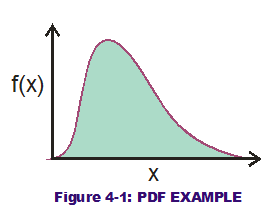
 What is a probability distribution? It is a mathematical representation of the likelihood for potential variable values to occur randomly over other possible values. More commonly, it is represented by the Probability Density Function (PDF), a mathematical function that models the probability density in histogram format. Displayed in Figure 4-1 is a rounded, hump-like curve over a range of possible variable values (along the x-axis). The height of the curve along the x-axis indicates a greater probability density for that particular value. It provides insight as to what values are more likely to occur. All possibilities should occur sometime if we sampled values to infinity and beyond. But some will occur more frequently than others. By using PDFs to represent the variation, as opposed to simple lower and upper bounds, the design engineer has made a great leap forward in understanding how to control variation of critical outputs.
There are many probability distributions that can be selected to model an input's variation. Frequently, there is not enough data or subject-matter expertise to select the appropriate distribution before Tolerance Analysis is performed. In the manufacturing world (as well as in many natural processes), the Normal distribution is king so baseline assumptions are typically made for normality behavior. (This can be dangerous in some circles but not so bad for dimensional ones.)
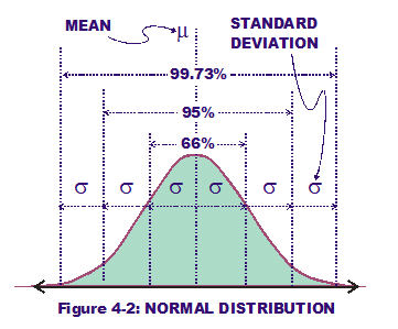
 It is defined by two PDF parameters, the mean and the standard deviation and is symmetrical (ie, non-skewed). The mean represents the central value; the engineer strives to center the mean of his observed production input values on the design-intent nominal dimensions. This places half of the possible dimension values to be greater than the mean and half to be less than the mean (symmetry). The other engineering goal would be to reduce (or control) the variation of the input by reducing the standard deviation, which is a "width" along the x-axis indicating the strength of the variance. Another cool property of the Normal distribution is that potential ranges along the x-axis have a cumulative probability associated with them, knowing how wide that range is in multiples of standard deviations (see Figure 4-2).
With this percentage-of-cumulative-probability concept associated with a range of variable values, we can estimate any range's cumulative probability using the two parameters' values, mean and standard deviation. (The key word here is "estimate." If the variable's behavior does not imitate normality, then we get further and further from the truth when using this estimation.) One particular range of interest is that which contains 99.73% of the variable's cumulative probability. That is the range contained within three standard deviations (or three "sigmas") on both sides of the mean. If a supplier can control dimensional variation where the 3-sigma range are within his spec limits (meaning 3 sigmas on both sides of the mean within LSL & USL), he is at least 3-sigma "capable." As a baseline, we assume most suppliers are at least 3-sigma capable, that they can keep their product performing within specs at least 99.73% of the time. (I will also use the 99.73%, 3-sigma range to estimate extreme values for RSS results, in order to have a decent "apples-to-apples" comparison against the WCA results.)
The magical world of RSS beckons. Yet we would be wise to understand the particulars of transfer functions and response surfaces and how that plays into RSS and Robust Design. (Permit me another side-bar in the next post.)
Breyfogle, Forrest W., Implementing Six Sigma: Smarter Solutions Using Statistical Methods (2nd ed) (2003); John Wiley & Sons, pp. 148-152.
Sleeper, Andrew D., Six Sigma Distribution Modeling (2006); McGraw-Hill, pp. 1-7.