 In my last couple of posts, I provided an introduction into the topic of Tolerance Analysis, relaying its importance in doing upfront homework before making physical products. I demonstrated the WCA method for calculating extreme gap value possibilities. Implicit in the underlying calculations was a transfer function (or mathematical relationship) between the system inputs and the output, between the independent variables and the dependent variable. In order to describe the other two methods of allocating tolerances, it is necessary to define and understand the underlying transfer functions.
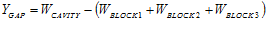
For the stacked block scenario (as in Figure 3-1), the system output of interest is the gap width between the righ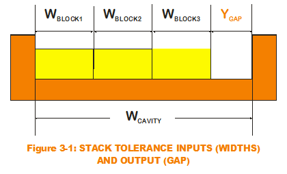 t end of the stacked blocks and the right edge of the U-shaped cavity. The inputs are the individual widths of each block and the overall cavity width. Simple addition and subtraction of the inputs results in the calculated output. Such is the case with all one-dimensional stack equations as can be seen with this transfer function:
Do all dimensional transfer functions look like this? It depends. Certainly, the one-dimensional stacks do. But let us also see how this might work with dimensional calculations of a two-dimensional nature.
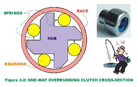 Consider the case of the overrunning or freewheel one-way clutch, a mechanism that allows a shaft or rotating component to rotate freely in one direction but not the other. Fishing reels use this mechanism to allow fish line to spool out freely in one direction but also allow the fish to be reeled in when rotating in the opposite direction. A typical cross-section of the one-way clutch is depicted in Figure 3-2. Primary components of the system are the hub and outer race (cylinder), connected by a common axis. They rotate freely with respect to each other, as wheels revolve around an axle. They also have internal contact via four cylindrical bearings that roll against both the outer surface of the hub and the inner surface of the race. The bearing contacts are kept in place with a series of springs that push the bearings into both the hub and race (springs are also in contact with hub). The end result is that the race rotates freely in one direction (counter-clockwise) but not the other (clockwise); thus the name.
The two system outputs of interest are the angle at which the bearings contact the outer race and the gap where the springs reside. Why are these two outputs important? To reduce shocks and jerks when contact is made during clockwise rotation, the design engineers must know where the rotation will stop and what potential variation exists around that stopping point. For the springs to have some nominal compression and maintain bearing position, a desired gap with some allowable variation needs to be defined. Neither of the two system outputs can be defined by a simple one-dimensional stack equation in that there are common input variables affecting both outputs simultaneously. The approach in defining the transfer functions, however, is the same. It is done by following a "closed loop" of physical locations (like contact points) through the system back to the original point, as a bunch of "stacked" vectors. Those vectors are broken down into their cartesian components which are the equivalent of two one-dimensional stacks. A more notable difference in the nature of the one-way clutch 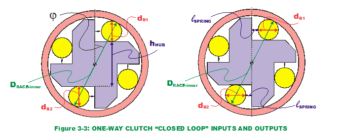 transfer functions versus those of the gap stack is their nonlinearities. Nonlinearities can introduce their unique influence to a transfer function. (But I digress.)
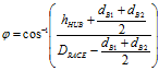
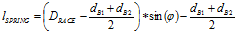
After some mathematical wrangling of the equations, the transfer functions for stop angle and spring gap are found to be:
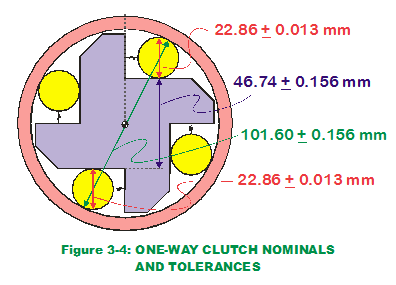 Let us apply the WCA approach and determine the extreme range of the outputs. (Figure 3-4 displays nominal and tolerance values for input dimensions in our transfer functions.) After some pondering the mechanical realities (or perhaps tinkering with high/low input values in the transfer functions), it can be seen that when the bearing diameters (dB1, dB2), the hub height (hHUB) and the race inner diameter (DCAGE) are at LMC limits, the contact angle (
 ) is at its extreme maximum value. Vice versa, if those same component dimensions are at MMC limits, the contact angle is at its extreme minimum value. The same exercise on spring gap brings similar results. Based on the information we know, the WCA approach results in these predicted extreme values for the two outputs:
|
OUTPUT
|
WCA Minimum Value
|
WCA Maximum Value
|
|
Stop Angle
|
27.380 ˚
|
28.371 ˚
|
|
Spring Gap (mm)
|
6.631
|
7.312
|
What is the allowable variation of the stop angle and spring gap? And do these minimum and maximum values fit within the customer-driven requirements for allowable variation?
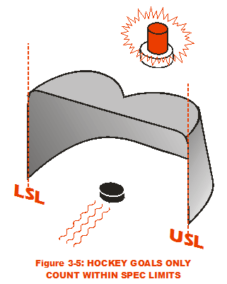 For design engineers, these requirements come on holy grails that glow in the dark; Specification Limits are inscribed on their marbled surfaces (cue background thunder). They are much like the vertical metal posts of a hockey goal crease. Any shots outside the limits do not ultimately satisfy the customer; they do not score a goal. These values will now be referred to as the Upper Specification Limit (USL) and the Lower Specification Limit (LSL). (Some outputs require either USL or LSL; not so for these outputs.) This table provides the specification limit values:
|
OUTPUT
|
LSL
|
USL
|
|
Stop Angle
|
27.50 ˚
|
28.50 ˚
|
|
Spring Gap (mm)
|
6.50
|
7.50
|
Comparing the WCA outcomes against the LSL/USL definitions, it appears we are in trouble with the stop angle. The extreme minimum value for stop angle falls below the LSL. What can be done? The power in the transfer functions is that it allows the design engineer to play "what-ifs" with input values and ensure the extreme WCA values fall within the LSL/USL values. If done sufficiently early in the design phase (before design "freezes"), the engineer has the choice of tinkering with either nominal values or their tolerances. Perhaps purchasing decisions to use off-the-shelf parts has locked in the nominal values to be considered but there is still leeway in changing the tolerances; in which case, the tinkering is done on only input tolerances. The opportunities for tinkering get fewer and fewer as product launch approaches so strike while the iron is hot.
How does this approach compare to the Root Sum Squares (RSS)? Before we explain RSS, it would be helpful to understand the basics of probability distributions, the properties of the normal distribution, and the nature of transfer functions and response surfaces (both linear and non-linear). So forgive me if I go off on a tangent into my next two posts. I promise I will come back to RSS after some brief digressions.
Creveling, Clyde M., Tolerance Design: A Handbook for Developing Optimal Specifications (1997); Addison Wesley Longman, pp. 111-117.