 Transfer Functions (or Response Equations) are useful to understand the "wherefores" of your system outputs. The danger with a good many is that they are not accurate. ("All models are wrong, some are useful.") Thankfully, the very nature of Tolerance Analysis variables (dimensions) makes the models considered here concrete and accurate enough. We can tinker with their input values (both nominals and variance) and determine what quality levels may be achieved with our system when judged against spec limits. That is some powerful stuff!
But beyond tinkering with input values, they are useful for understanding the underlying nature of the engineered system and guiding future design decisions in a highly effective fashion. When the nature of the transfer function is understood, along with its design-peculiar nonlinearities or curvature, it opens or closes more avenues for design exploration to the engineer. Always a good thing to learn this up front.
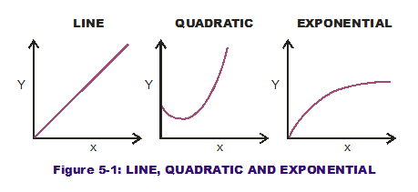
 Examine the transfer functions depicted as graphical curves in Figure 5-1. All of them represent one output (Y) on the vertical axis while the horizontal represents one input (x). The first two are the well-known linear and quadratic polynomial equations (line and parabola) while the last is an exponential. Many texts would indicate the second curve to be "non-linear" and since it does not resemble a line, there is a certain truth to that. But I much prefer calling the quadratic a linear combination higher-order terms (squared, cubed, etc…) of the baseline linear terms, output proportional to input, without any exponentiation. Non-linear (when I use it here without quotes) represents just about everything else except the polynomials (linear combination of first- and higher-order terms). Like the exponential curve or inverse cosines (like stop angle in the one-way clutch).
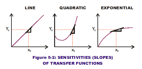
 Let us assume that each of these curves represents a different design solution where a particular output response (Y0) is desired (see Figure 5-2). The plots are shown in the same scales for both inputs and outputs. Also, for simplicity, we will assume there is no variation in the design input value selected (even though we know that assumption is false). If the middle value of the input along the x-axis is selected for all three curves (x0) and that results in a corresponding output value that is the same for all three, which design is better than the rest?
Assuming there is no variation in the input, there is no difference associated with this output across all three designs. But if there is variation in the input, the answer is very different. The distinguishing aspect of the three curves is in their slopes at the design point of interest. The slope of a curve can be expressed as the first derivative of the output with respect to the input of concern. The greater this value is at the design point of interest, the greater the slope and thus the greater the sensitivity is to that input variable. For our design to be robust to the inherent variation in any input variable, we desire a lesser sensitivity with respect to that variable. This will become apparent with the RSS and Monte Carlo methodologies.
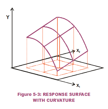
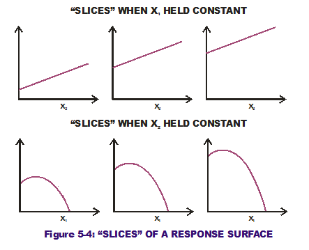
 Now let us examine a transfer function with two inputs to a singular output (Figure 5-3). Instead of representing the function with a line or curve and the two axes (input to output), it is now represented as a surface in three-dimensional space which undulates at various heights over a two-dimensional surface. The flat level surface at the bottom represents two inputs whose values must be "frozen" in the design phase. Because of this representation, these are usually termed Response Surfaces. Note that if a design decision has been made to "freeze" the nominal value of one input variable (in effect, "slicing" the surface while holding that input constant), the resulting slice of the Response Surface is back to a one-output-to-one-input line or curve. Thusly, we could take "slices" of the Response Surface and plot those as lines or curves. Figure 5-4 shows the results when we hold the first input (x1) constant at three different values and when we hold the second input (x2) constant at three different values. This produces six curves. Note that by holding x1 constant, all three lines produced have the same slope over the entire range of x2 values of concern. This is true despite the height of the curves being different (greater nominal response when x1 is held constant at the greater values). The sensitivity of the output to x2 is the same no matter what values of x1 or x2 are chosen.
The same cannot be said of sensitivity of the output to x1. When x2 is held constant, the "slices" produced are quadratic, second-order polynomials. So our output is very sensitive to the design decision made on the first input, x1. With no other considerations in mind (and keep in mind there probably are others), the design e ngineer may be inclined to select the x1 input value that results in zero slope (as in at the top of the parabolas shown). This minimizes Sensitivity with respect to that variable. Doing this across all variables should result in a Robust Design (robust as much as possible to the input variations).
I have laid some groundwork for understanding the Root Sum Squares approach while performing Tolerance Analysis. Stay tuned over the next couple of posts as we explore the magical world of RSS.
Creveling, Clyde M., Tolerance Design: A Handbook for Developing Optimal Specifications (1997); Addison Wesley Longman, pp. 149-159.
Myers, R.H. and Montgomery, D.C., Response Surface Methodology: Process and Product Optimization Using Designed Experiments (1995); John Wiley & Sons, pp. 208-214.