Engineering Modeling

Discrete Distribution Fitting to Duke Basketball Scores, in ModelRisk (4/8)

Eric Torkia, MASc

Share:

Print

Rate article:

No rating
Rate this article:
No rating

Let the battle begin anew. We continue our journey in uncertainty modeling, having understood how to fit distributions to data using Crystal Ball (CB). How does that experience compare to what ModelRisk (MR) has to offer?

Open the Duke 09_10 Scores spreadsheet with ModelRisk loaded in the Excel environment. We will first create the MR Objects representing the fitted PDFs. (Just as with the CB exercise, it is good practice to examine a variety of best-fitting distributions, rather than blindly accepting the top dog.) Then, in distinctly separate cells, we will create the VoseSimulate functions that behave as sampled values from the PDFs modeled by the MR Objects.

  •  Select "Fit" button in the ModelRisk ribbon bar. (This opens the Distribution Fitting window. It does not matter which cell has been selected before clicking "Fit" button.)
  • Select "Distribution Fit" in the drop-down list.
  • Identify the "Data Location:" (upper left-hand corner) as Cells C4:C37.


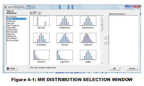
  • Select "Add" button (just below "Data location:" and "Truncated" enable box). (The PDF selection window will appear; see Fig. 4-1.)
  • Select "Discrete" within "Type of Distribution" list (left-hand side).
  • Individually select the first 11 distributions using CTL key.
  • Select double right arrow (">>") button to place the identified distributions into right-hand column list.
  • Select "OK."

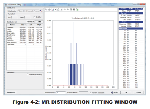
What appears next will be the user-friendly distribution-fitting window for MR with ranked distributions listed on the left-hand side (see Fig. 4-2). On the left-hand side are the distributions selected for fitting. They are ranked from top-to-bottom in order of best fits. Note that the criteria (SIC, AIC and HQIC) are not the same as used in CB (Chi-squared). And for good reason. These criteria penalize some fits as being less worthy if more parameters are used for the fitting. Just like with regression or ANOVA work, additional terms can be added for a better fit but that is a reflection of, perhaps, an unnecessarily-complex model. Simpler is better in many cases. Even with "over-fitting" penalties, the top-most distributions have two or more parameters, indicating the greater flexibility is desirable.

Now we will place both the MR Object and the PDF parameters into the spreadsheet.

  • Select first distribution listed on left-hand side ("Delaporte").
  • Select 'Excel-with-plus-sign' (right-most) icon above the histogram.
  • Select "Parameters" from drop-down menu.
  • Select Cells R4:T5.
  • Select "OK." (These steps place the PDF parameters into the designated cells.)
  • Select 'Excel-with-plus-sign' icon (again) above the histogram.
  • Select "Object" from drop-down menu.
  • Select Cell U5.
  • Select "OK." (These steps place the MR Object into the designated cell.)

Of interest are the next four best-fitting distributions. Follow the same steps above for the next four PDFs. Before selecting the 'Excel-with-plus-sign' icon, select the next best distribution in the left-hand-side list. Parameters and Objects for the remaining four best-fitting distributions can be placed in the following cells:

2) PolyA - Parameters in R6:S7, Object in U7

3) NegBin- Parameters in R8:S9, Object in U9

4) BetaNegBin - parameters in R10:T11, Object in U11

5) BetaBinomial - parameters in R12:T13, Object in U13

After these five sets of parameters and Objects have been created, select "OK" to exit distribution-fitting window.

The final touch is to create cells that behave like uncertain input variables in Excel. We place the VoseSimulate function into the model architecture (input) and refer back to the fitted-distribution Objects.

  • Select Cell P5.
  • Type in "=VoseSimulate(U5)" and hit ENTER. (Or use Formula Bar tool to do the same).
  • Copy Cell P5.
  • Paste the formula into Cells P7, P9, P11, and P13.

We leave it to the reader to complete the exercise for the Opponent's Score in the rows directly beneath.

(After entering the MR enablers in Column P, single trials can be experienced if automatic recalculation is "on" in Excel (via Excel Options) and any changes are made elsewhere in the sheet. Try it out by typing a number in any blank cell and hitting ENTER.)

What becomes apparent immediately, in the ModelRisk world, is that we have a lot more options available for distribution-fitting. And do we, as self-appointed basketball experts, believe that these new alternatives are perhaps even better offerings than what Crystal Ball provided?


We do. PolyA is a modification of Poisson. Even better, PolyA substitutes the Gamma distribution (defined by two parameters) for the Rate parameter, allowing us to be uncertain about the actual scoring rate mean for each game. Perfect! Also helpful is Delaporte. It takes the PolyA modification of the Poisson even further, combining a static element (Rate) with an uncertain one (Gamma distribution & its two parameters) and subs that in for the Poisson Rate parameter. Also interesting are the Beta Negative Binomial and Beta Binomial. As you would suspect, they are modifications of the Binomial and Negative Binomial. Just like the Gamma distribution was used in Poisson, the Beta distribution is subbed in for the Probability parameter, placing uncertainty around the coin flip probabilities from game to game.

These are not the only reasons to be excited about discrete distribution fitting in MR. Another great bonus over CB fitting is that the data need not be static. There is no automatic feature in CB that updates CB Assumptions fitted to that data. The fitting operation needs to be manually run again to obtain a new set of PDF parameters. In MR, the user just needs to insert extra cells in the data ranges and all appropriate Vose formulas are updated, just like with Excel formulas. Voila!

Lastly, it should be mentioned that MR trumps CB in another important distribution-fitting category. MR allows the user to fit to the minimum number of samples necessary to calculate PDF MLEs. This can be a dangerous thing in the hands of a novice. MR guards against that danger by incorporating an uncertainty parameter in Vose functions. In contrast, CB places a minimum limit of 15 on the number of samples to be fitted. For those with frequent low number of samples, this is a major hindrance. We will return to this topic in the future.

There is one important tweak we have not placed on either of our CB or MR entities. Now we turn our attention to the added complication of correlations.

Comments

Collapse Expand Comments (0)
You don't have permission to post comments.

Oracle Crystal Ball Spreadsheet Functions For Use in Microsoft Excel Models

Oracle Crystal Ball has a complete set of functions that allows a modeler to extract information from both inputs (assumptions) and outputs (forecast). Used the right way, these special Crystal Ball functions can enable a whole new level of analytics that can feed other models (or subcomponents of the major model).

Understanding these is a must for anybody who is looking to use the developer kit.

Why are analytics so important for the virtual organization? Read these quotes.

Jun 26 2013
6
0

Since the mid-1990s academics and business leaders have been striving to focus their businesses on what is profitable and either partnering or outsourcing the rest. I have assembled a long list of quotes that define what a virtual organization is and why it's different than conventional organizations. The point of looking at these quotes is to demonstrate that none of these models or definitions can adequately be achieved without some heavy analytics and integration of both IT (the wire, the boxes and now the cloud's virtual machines) and IS - Information Systems (Applications) with other stakeholder systems and processes. Up till recently it could be argued that these things can and could be done because we had the technology. But the reality is, unless you were an Amazon, e-Bay or Dell, most firms did not necessarily have the money or the know-how to invest in these types of inovations.

With the proliferation of cloud services, we are finding new and cheaper ways to do things that put these strategies in the reach of more managers and smaller organizations. Everything is game... even the phone system can be handled by the cloud. Ok, I digress, Check out the following quotes and imagine being able to pull these off without analytics.

The next posts will treat some of the tools and technologies that are available to make these business strategies viable.

Multi-Dimensional Portfolio Optimization with @RISK

Jun 28 2012
16
0

Many speak of organizational alignment, but how many tell you how to do it? Others present only the financial aspects of portfolio optimization but abstract from how this enables the organization to meets its business objectives.  We are going to present a practical method that enables organizations to quickly build and optimize a portfolio of initiatives based on multiple quantitative and qualitative dimensions: Revenue Potential, Value of Information, Financial & Operational Viability and Strategic Fit. 
                  
This webinar is going to present these approaches and how they can be combined to improve both tactical and strategic decision making. We will also cover how this approach can dramatically improve organizational focus and overall business performance.

We will discuss these topics as well as present practical models and applications using @RISK.

Reducing Project Costs and Risks with Oracle Primavera Risk Analysis

.It is a well-known fact that many projects fail to meet some or all of their objectives because some risks were either: underestimated, not quantified or unaccounted for. It is the objective of every project manager and risk analysis to ensure that the project that is delivered is the one that was expected. With the right know-how and the right tools, this can easily be achieved on projects of almost any size. We are going to present a quick primer on project risk analysis and how it can positively impact the bottom line. We are also going to show you how Primavera Risk Analysis can quickly identify risks and performance drivers that if managed correctly will enable organizations to meet or exceed project delivery expectations.

.


Modeling Time-Series Forecasts with @RISK


Making decisions for the future is becoming harder and harder because of the ever increasing sources and rate of uncertainty that can impact the final outcome of a project or investment. Several tools have proven instrumental in assisting managers and decision makers tackle this: Time Series Forecasting, Judgmental Forecasting and Simulation.  

This webinar is going to present these approaches and how they can be combined to improve both tactical and strategic decision making. We will also cover the role of analytics in the organization and how it has evolved over time to give participants strategies to mobilize analytics talent within the firm.  

We will discuss these topics as well as present practical models and applications using @RISK.

The Need for Speed: A performance comparison of Crystal Ball, ModelRisk, @RISK and Risk Solver


Need for SpeedA detailed comparison of the top Monte-Carlo Simulation Tools for Microsoft Excel

There are very few performance comparisons available when considering the acquisition of an Excel-based Monte Carlo solution. It is with this in mind and a bit of intellectual curiosity that we decided to evaluate Oracle Crystal Ball, Palisade @Risk, Vose ModelRisk and Frontline Risk Solver in terms of speed, accuracy and precision. We ran over 20 individual tests and 64 million trials to prepare comprehensive comparison of the top Monte-Carlo Tools.


Excel Simulation Show-Down Part 3: Correlating Distributions

Escel Simulation Showdown Part 3: Correlating DistributionsModeling in Excel or with any other tool for that matter is defined as the visual and/or mathematical representation of a set of relationships. Correlation is about defining the strength of a relationship. Between a model and correlation analysis, we are able to come much closer in replicating the true behavior and potential outcomes of the problem / question we are analyzing. Correlation is the bread and butter of any serious analyst seeking to analyze risk or gain insight into the future.

Given that correlation has such a big impact on the answers and analysis we are conducting, it therefore makes a lot of sense to cover how to apply correlation in the various simulation tools. Correlation is also a key tenement of time series forecasting…but that is another story.

In this article, we are going to build a simple correlated returns model using our usual suspects (Oracle Crystal Ball, Palisade @RISK , Vose ModelRisk and RiskSolver). The objective of the correlated returns model is to take into account the relationship (correlation) of how the selected asset classes move together. Does asset B go up or down when asset A goes up – and by how much? At the end of the day, correlating variables ensures your model will behave correctly and within the realm of the possible.

Copulas Vs. Correlation

Copulas and Rank Order Correlation are two ways to model and/or explain the dependence between 2 or more variables. Historically used in biology and epidemiology, copulas have gained acceptance and prominence in the financial services sector.

In this article we are going to untangle what correlation and copulas are and how they relate to each other. In order to prepare a summary overview, I had to read painfully dry material… but the results is a practical guide to understanding copulas and when you should consider them. I lay no claim to being a stats expert or mathematician… just a risk analysis professional. So my approach to this will be pragmatic. Tools used for the article and demo models are Oracle Crystal Ball 11.1.2.1. and ModelRisk Industrial 4.0

Excel Simulation Show-Down Part 2: Distribution Fitting


One of the cool things about professional Monte-Carlo Simulation tools is that they offer the ability to fit data. Fitting enables a modeler to condensate large data sets into representative distributions by estimating the parameters and shape of the data as well as suggest which distributions (using these estimated parameters) replicates the data set best.

Fitting data is a delicate and very math intensive process, especially when you get into larger data sets. As usual, the presence of automation has made us drop our guard on the seriousness of the process and the implications of a poorly executed fitting process/decision. The other consequence of automating distribution fitting is that the importance of sound judgment when validating and selecting fit recommendations (using the Goodness-of-fit statistics) is forsaken for blind trust in the results of a fitting tool.

Now that I have given you the caveat emptor regarding fitting, we are going to see how each tools offers the support for modelers to make the right decisions. For this reason, we have created a series of videos showing comparing how each tool is used to fit historical data to a model / spreadsheet. Our focus will be on :

The goal of this comparison is to see how each tool handles this critical modeling feature.  We have not concerned ourselves with the relative precision of fitting engines because that would lead us down a rabbit hole very quickly – particularly when you want to be empirically fair.

RESEARCH ARTICLES | RISK + CRYSTAL BALL + ANALYTICS