 Are there discrete univariate probability distribution functions (PDFs) that can be used to simulate college basketball scores? Do we, as avid basketball observers, know enough to suggest one discrete PDF is better than another? In fitting distributions to data in your business problems, the analyst will be asking the same types of questions. If the analyst is not an expert on the inputs and their behavior, he or she should seek out a subject-matter expert (SME) who can provide insight. Putting experience and theoretical knowledge together this way is a best practice for distribution selection.
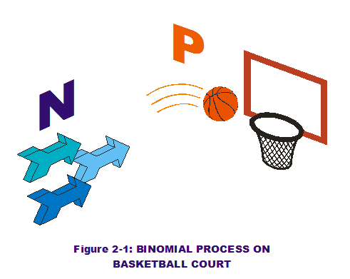
Out of the four best-fitting PDF candidates for Duke's game scores, the first three do make sense to use. The Binomial and Negative Binomial distributions, for instance, are appropriate in modeling basketball scores. Why? Both are used in modeling Binomial Processes, where a progressive series of "coin flips" are made. It represents a defined number of trials of individual coin flips (N, or # of Trials) that can either fail (# of Failures) or succeed (# of Successes). The coin is weighted with the probability, P, of a success. Nitpicky statisticians would point out the Shape factor, S, represents the number of successes when predicting the number of failures to occur before the r-th success. These are the parameters for the Negative Binomial. What about the Binomial distribution? It represents the number of successes achieved in N flips of coin with probability P.

Why does the Binomial process matter to basketball games? It could be said that each trip up the court represents a scoring opportunity or a coin flip. Each team has a unique ability to affect their own probability of success throughout an entire game or season. Each trip up the court is an opportunity to test that probability. It is true that each flip is (usually) 2 points, a potential argument against using the Binomial process PDFs. Another con is that both assume a precise number of trials, N, which is not the case. Variation exists in N from game-to-game. Is there a method to account for that?
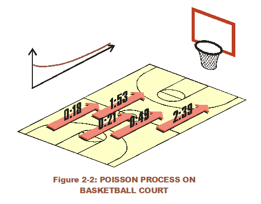
From a similar viewpoint, the Poisson makes sense, perhaps even better. The Poisson process models a sequential event process (much like coin flips) that occur in a set time. However, it is not a matter of success or failure per flip. It is simply a matter of when the coin gets flipped. There is variation with between-time, between events (or flips) occuring. The distribution associated with time between arrivals (Exponential) is continuous while the Poisson distribution is discrete. The Poisson could represent the number of times a college basketball team scores within 48 minutes, or the number of arrivals in a set time.

Despite its rank within the top four, (and noting its separation from Geometric via the Chi-Square criterion), the Discrete Uniform seems unlikely. It is the discrete univariate brother of the continuous univariate Uniform distribution. While useful in describing an expert's opinion about a range of potential values, the Uniform places no weighting of some values over another. Instead, all values are equally probable, generally resulting in over-conservative MCA results. It is the last line of defense in estimating variable uncertainty, true. But it makes no immediate sense for a college basketball output. We will concentrate future distribution-selection efforts around the Binomial or the Poisson Process.
It is safe to say that the distribution-selection process is a mixture of calculated criteria, statistical knowledge and experience. The CB distribution-fitting criterion takes care of the first part. The user should recognize the PDF alternatives and compare their intended use with what their experience tells them. Then make a balanced judgment call. Subject Matter Experts (SME) are an important component in modeling input variation accurately and should always be consulted before hitting the "Run" button.