 How do Monte Carlo analysis results differ from those derived via WCA or RSS methodologies? Let us return to the one-way clutch example and provide a practical comparison in terms of a non-linear response. From the previous posts, we recall that there are two system outputs of interest: stop angle and spring gap. These outputs are described mathematically with response equations, as transfer functions of the inputs.
What options are there to run Monte Carlo (MC) analysis on our laptops? There are quite a few (a topic that invites a separate post). For the everyday user, it makes good sense to utilize one that works with existing spreadsheet logic, as in an Excel file. There are three movers and shakers in the Monte Carlo spreadsheet world which one might consider: Crystal Ball, ModelRisk and @Risk. (If you examine our offerings, www.crystalballservices.com, you will find we sell the first two.) For the purposes of this series, we will use Crystal Ball (CB) but will return to ModelRisk in the near future.
As with the RSS approach, it makes sense to enter the transfer function logic into an Excel spreadsheet where equations define the system output as linked to the inputs located in other cells. (Please refer to the "One-Way Clutch with Monte Carlo" spreadsheet model in our model archives. Figure 11-1 contains a snapshot of this spreadsheet.) The inputs and outputs are arrang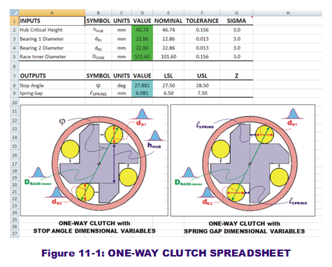 ed in vertical order. Each of the inputs has a nominal and tolerance value associated with them, along with a desired Sigma level. As stated in previous posts, it will be assumed the suppliers of these inputs are 3-sigma capable and that their behaviors are normally distributed. Going forward, this means the standard deviations are assumed to be one-third of the tolerance value.
The noticeable difference between this spreadsheet and the previous one (focused only on WCA and RSS results) is the coloring of the cells in the column titles "Values." The input "values" are colored green while the output "values" are colored blue. In the Crystal Ball (CB) world, these colors indicate a probabilistic behavior has been assigned to these variables. If we click on one of the green cells and then the "Define Assumption" button in the CD ribbon bar, a dialog box opens to reveal which distribution was defined for that input. The user will find that they are all normal distributions and the parameters (mean and stdev) are cell-referenced to the adjacent "Nominal," "Tolerance" and "Sigma" cells within the same row. (Note the standard deviation is calculated as the tolerance divided by the sigma. If this is not visible in your CB windows, hit CTL-~.)
We can run the simulation as is. But before we do, an important MC modeling distinction should be made. In the RSS derivations, we assumed that the contributive nature of both bearings (bought in batches from the same supplier) were equal and therefore assumed the same variable behavior for both diameters as one singular variable (dB1) in the output transfer functions. However, this assumption in the transfer function should not be used for the transfer functions in the Monte Carlo analysis.
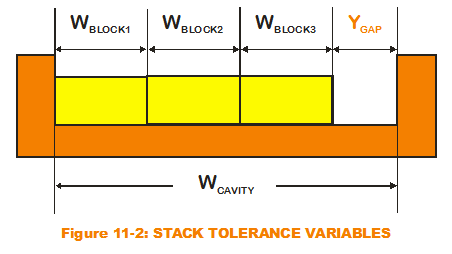 Re-examine the case of the classic stack-up tolerance example from my first few posts (see Figure 11-2). Note that for the transfer function, I have distinguished each block width as a separate input variable. Had I assumed the same input variable for all three (so that the output gap transfer function is cavity width minus three times a singular block width), I would have invited disaster. Explicit in the incorrect transfer function is an assumption that all three block widths will vary in synchronicity. If the block width is randomly chosen as greater than the nominal by the MC simulation, all three block widths would be artificially larger than their nominals. Obviously, this is not what would happen in reality. The simulation results would overpredict variation. Therefore, the MC modeler must assign different variables for all block widths, even though the probability distributions that define their variation are one and the same.
To run the simulation, the user simply clicks on the "Start" button in the CB ribbon bar. Immediately obvious should be the CB Forecast windows that pop up in the forefront to display the simulation as it runs. The visual result is output histograms that show the variation with respect to the spec limits (LSL & USL), as seen in Figure 11-3. CB 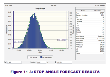 also can place particular output results values (such as mean, stdev, capability metrics and percentiles) into defined cells (Cells I12:AK13) via Forecast options.
Here is the moment of truth. How did MC analysis compare to the WCA and RSS results? For an even better "apples-to-apples" comparison, the analyst may decide to extract percentiles associated with the 99.73% range (3 sigmas to either side), rather than calculate them from mean and standard deviation. If there is any non-normal behavior associated with the output, MC analysis can extract the values corresponding to the 3-sigma range, providing more accuracy on the extreme range despite non-normality. The same cannot be said of either WCA or RSS. ("Min Values" and "Max Values" for all three methods are displayed in Columns J & K.)
Figure 11-4 summarizes the range comparisons on both system outputs for the three methods. Surprisingly enough, MC provides a wider range of stop angle extreme values than RSS but less wide than the conservative WCA approach. (RSS and 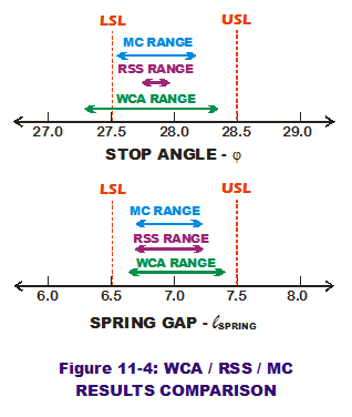 MC agree pretty much on spring gap range while still being less than the WCA range.) The reason for the difference in stop angle extreme ranges is related to a difference in predicted standard deviations. The MC method predicts an output standard deviation that is two orders of magnitude greater than the RSS output standard deviation. (Your results may vary based on number of trials and random seed values but should be approximately the same.) The approximations based in RSS scribes can sometimes be too relaxed, especially if linearity and normality assumptions are violated. They can be too liberal and would paint a rosy picture for dimensional quality predictions.
Is that the only reason to prefer MC analysis over RSS? Follow my next post as we revisit the topic of sensitivities and sensitivity contributions as they apply in the MC world.
Creveling, Clyde M., Tolerance Design: A Handbook for Developing Optimal Specifications (1997); Addison Wesley Longman, pp. 163-167.