As stated before, the first derivative of the transfer function with respect to a particular input quantifies how sensitive the output is to that input. However, it is important to recognize that Sensitivity does not equal Sensitivity Contribution. To assign a percentage variation contribution from any one input, one must look towards the RSS output variance (σ_Y²) equation:

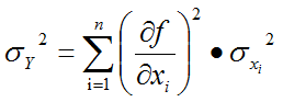
Note that the variance is the sum product of the individual input variances (σ_xi²) times their Sensitivities (1^st derivatives) squared. Those summed terms represent the entirety of each input's variation contribution. Therefore, it makes sense to divide individual terms (product of variance and sensitivity squared) by the overall variance. Running the calculation this way ensures the total will always add up to 100%. (BTW: The results are included in an Excel spreadsheet titled "One-Way Clutch with RSS" from our file archives.  To download this file is available for all registered users who have logged in.  If you have not currently logged in, this link will direct to our quick login/registration page.)

After the dust settles, the end result for the two output means and standard deviations are:

We can use these mean and standard deviation values to estimate the 99.73% range and use these extreme range values to be an "apples-to-apples" comparison against the WCA results. Those values, standing at three standard deviations on either side of the predicted mean are:

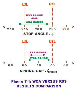How do these extreme results compare to WCA values? And how do each of them compare to the LSL & USL, respectively? Figure 7-1 plots the three pairs of values to make visual comparisons.

RSS predicts both extreme values for stop angle to be within the spec limits; WCA does not. Not only does WCA place both of its predicted extreme values further out than RSS does, one of them is lower than LSL (which is a bad thing). Why? The reason is that RSS accounts for the joint probability of two or more input values occurring simultaneously accurately while WCA does not. In the WCA world, any input value has equal merit to any other, as long as it is in the bounds of the tolerance. It is as if a uniform probability distribution has been used to describe their probability of occurrence. RSS says "not so." It accounts for the unlikely joint probability that those extreme combinations of values are much less likely to occur than the central tendency combinations. Thus, RSS is much less conservative than WCA and also more accurate.

Another big distinction between the two approaches is that RSS provides sensitivity and sensitivity contribution values according to each input while WCA does not. Sensitivities and contributions allow the engineer to quantify which input variables are variation drivers (and which ones are not). Thus, a game plan can be devised to reduce or control variation on the drivers that matter (and eliminate those drivers that do not from any long-winded control plan). The sensitivity information is highly valuable in directing the design activities focused on variation to the areas that need it. It makes design engineering that more efficient.

A summary of pros and cons when comparing WCA against RSS:

Perhaps RSS is the clear winner? Not if you lack a penchant for doing calculus. Not if your transfer function is highly non-linear. Before we progress to Monte Carlo analysis, let us step back and develop a firm understanding of the RSS equations. In my next post, I will illustrate the RSS properties in graphical format because pictures are worth a thousand words.

Creveling, Clyde M., Tolerance Design: A Handbook for Developing Optimal Specifications (1997); Addison Wesley Longman, pp. 126-147.

Hahn, G.J. and Shapiro S.S. (1994), Statistical Models in Engineering; J Wiley and Sons, pp. 252-255.

Sleeper, Andrew D., Design for Six Sigma Statistics (2006); McGraw-Hill, pp. 716-730.