Engineering Modeling

Root Sum Squares Explained Graphically (Part 8 / 13)

Karl - CB Expert

Share:

Print

Rate article:

5.0
Rate this article:
5.0

A few posts ago, I explained the nature of transfer functions and response surfaces and how they impact variational studies when non-linearities are concerned. Now that we have the context of the RSS equations in hand, let us examine the behavior of transfer functions more thoroughly.

Sensitivities are simply the slope values (1st derivatives) of the transfer functions. If I take "slices" of a two-inputs-to-one-output of the response surface, I can view the sensitivities (slopes) along those slices. But why are steeper slopes considered more sensitive?

Examine Figure 8-1. It shows three mathematical representations of a one-input-to-one-output transfer function. These curves (all straight lines) represent three different design solutions under consideration. When the designer selects the mid-point of the horizontal axis as his design input value (x0), all three transfer functions provide the same output (Y0) response value along the vertical axis. What makes one better than the others?

Now examine Figure 8-2. We have added a 
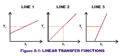
variational component to the input values in the form of a normal curve along the horizontal axes. Remember that the height of the PDF shown indicates some values are more likely to occur than others. The variability shown in the input can be transferred to the output variation through the transfer function curve. For the first line, this results in a normal curve on the response with a known standard deviation (as shown on the vertical axis). For the second line, this also results in a normal curve but one that has a wider range of variation (a larger standard deviation). For the third and steepest line, we get another normal curve with an even greater range of variation. The first line (or design solutio
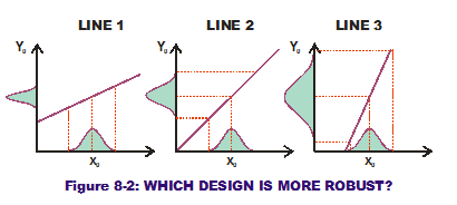
n under consideration) produces less variation (less noise) on the output when input variation is same for all three scenarios. It is a more Robust Design than the other two (less sensitive to noise in the input variations).


What if there are multiple inputs to our one output? Does one input's variation wreak more havoc than another input's variation? This is the question that Sensitivity Contribution attempts to answer. Consider the response surface in Figure 8-3, a completely flat surface that is 
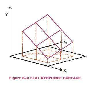
angled to the horizontal plane (not level). Figure 8-4 displays the slices we cut while holding x1 constant at different values and doing the same for x2. Note that the slopes (which are constant and do not change over the input range of interest) are of a lesser magnitude when x1 is held constant versus when x2 is held constant. That means the response is less sensitive to variation in the second input (x2) than the first input (x1). (As a side note: The steeper slices, when x2 is held constant, have a negative sign indicating a downward slope.)

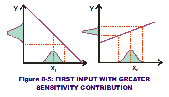
If we apply the same variation to both x1 and x2 (see Figure 8-5), it is obvious that the first input causes greater output variation. Therefore, it has a greater sensitivity contribution than that of the second input.


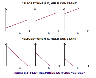
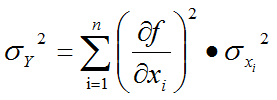
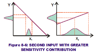
We can flip the tables, however. What if the variation of x2 was so much greater than that of x1? (See Figure 8-6.) It is possible that, after the variation of x1 and x2 have been "transferred" through the slopes, that the corresponding output variation due to x2 is greater than that from x1. Now the second input (x2) has a greater sensitivity contribution component than the first input (x1), even though the first input has a greater sensitivity than the second input. By examining the RSS equation for output variance (see below), it can be seen why this is the case.


If either the slopes (1st derivatives) of a design solution of interest or the variation applied to those slopes (the input standard deviations) is increased, that input's sensitivity contribution goes up while all the others go down. The pie must equal 100%.

So we now know how much pie there is to allocate to the individual input tolerances, being based on the sensitivities and input variations. Let us stop eating pie for the moment and look at the other RSS equation, that of predicted output mean. (RSS is really easy to understand if you look at it graphically.)

Comments

Collapse Expand Comments (0)
You don't have permission to post comments.

Oracle Crystal Ball Spreadsheet Functions For Use in Microsoft Excel Models

Oracle Crystal Ball has a complete set of functions that allows a modeler to extract information from both inputs (assumptions) and outputs (forecast). Used the right way, these special Crystal Ball functions can enable a whole new level of analytics that can feed other models (or subcomponents of the major model).

Understanding these is a must for anybody who is looking to use the developer kit.

Why are analytics so important for the virtual organization? Read these quotes.

Jun 26 2013
6
0

Since the mid-1990s academics and business leaders have been striving to focus their businesses on what is profitable and either partnering or outsourcing the rest. I have assembled a long list of quotes that define what a virtual organization is and why it's different than conventional organizations. The point of looking at these quotes is to demonstrate that none of these models or definitions can adequately be achieved without some heavy analytics and integration of both IT (the wire, the boxes and now the cloud's virtual machines) and IS - Information Systems (Applications) with other stakeholder systems and processes. Up till recently it could be argued that these things can and could be done because we had the technology. But the reality is, unless you were an Amazon, e-Bay or Dell, most firms did not necessarily have the money or the know-how to invest in these types of inovations.

With the proliferation of cloud services, we are finding new and cheaper ways to do things that put these strategies in the reach of more managers and smaller organizations. Everything is game... even the phone system can be handled by the cloud. Ok, I digress, Check out the following quotes and imagine being able to pull these off without analytics.

The next posts will treat some of the tools and technologies that are available to make these business strategies viable.

Multi-Dimensional Portfolio Optimization with @RISK

Jun 28 2012
16
0

Many speak of organizational alignment, but how many tell you how to do it? Others present only the financial aspects of portfolio optimization but abstract from how this enables the organization to meets its business objectives.  We are going to present a practical method that enables organizations to quickly build and optimize a portfolio of initiatives based on multiple quantitative and qualitative dimensions: Revenue Potential, Value of Information, Financial & Operational Viability and Strategic Fit. 
                  
This webinar is going to present these approaches and how they can be combined to improve both tactical and strategic decision making. We will also cover how this approach can dramatically improve organizational focus and overall business performance.

We will discuss these topics as well as present practical models and applications using @RISK.

Reducing Project Costs and Risks with Oracle Primavera Risk Analysis

.It is a well-known fact that many projects fail to meet some or all of their objectives because some risks were either: underestimated, not quantified or unaccounted for. It is the objective of every project manager and risk analysis to ensure that the project that is delivered is the one that was expected. With the right know-how and the right tools, this can easily be achieved on projects of almost any size. We are going to present a quick primer on project risk analysis and how it can positively impact the bottom line. We are also going to show you how Primavera Risk Analysis can quickly identify risks and performance drivers that if managed correctly will enable organizations to meet or exceed project delivery expectations.

.


Modeling Time-Series Forecasts with @RISK


Making decisions for the future is becoming harder and harder because of the ever increasing sources and rate of uncertainty that can impact the final outcome of a project or investment. Several tools have proven instrumental in assisting managers and decision makers tackle this: Time Series Forecasting, Judgmental Forecasting and Simulation.  

This webinar is going to present these approaches and how they can be combined to improve both tactical and strategic decision making. We will also cover the role of analytics in the organization and how it has evolved over time to give participants strategies to mobilize analytics talent within the firm.  

We will discuss these topics as well as present practical models and applications using @RISK.

The Need for Speed: A performance comparison of Crystal Ball, ModelRisk, @RISK and Risk Solver


Need for SpeedA detailed comparison of the top Monte-Carlo Simulation Tools for Microsoft Excel

There are very few performance comparisons available when considering the acquisition of an Excel-based Monte Carlo solution. It is with this in mind and a bit of intellectual curiosity that we decided to evaluate Oracle Crystal Ball, Palisade @Risk, Vose ModelRisk and Frontline Risk Solver in terms of speed, accuracy and precision. We ran over 20 individual tests and 64 million trials to prepare comprehensive comparison of the top Monte-Carlo Tools.


Excel Simulation Show-Down Part 3: Correlating Distributions

Escel Simulation Showdown Part 3: Correlating DistributionsModeling in Excel or with any other tool for that matter is defined as the visual and/or mathematical representation of a set of relationships. Correlation is about defining the strength of a relationship. Between a model and correlation analysis, we are able to come much closer in replicating the true behavior and potential outcomes of the problem / question we are analyzing. Correlation is the bread and butter of any serious analyst seeking to analyze risk or gain insight into the future.

Given that correlation has such a big impact on the answers and analysis we are conducting, it therefore makes a lot of sense to cover how to apply correlation in the various simulation tools. Correlation is also a key tenement of time series forecasting…but that is another story.

In this article, we are going to build a simple correlated returns model using our usual suspects (Oracle Crystal Ball, Palisade @RISK , Vose ModelRisk and RiskSolver). The objective of the correlated returns model is to take into account the relationship (correlation) of how the selected asset classes move together. Does asset B go up or down when asset A goes up – and by how much? At the end of the day, correlating variables ensures your model will behave correctly and within the realm of the possible.

Copulas Vs. Correlation

Copulas and Rank Order Correlation are two ways to model and/or explain the dependence between 2 or more variables. Historically used in biology and epidemiology, copulas have gained acceptance and prominence in the financial services sector.

In this article we are going to untangle what correlation and copulas are and how they relate to each other. In order to prepare a summary overview, I had to read painfully dry material… but the results is a practical guide to understanding copulas and when you should consider them. I lay no claim to being a stats expert or mathematician… just a risk analysis professional. So my approach to this will be pragmatic. Tools used for the article and demo models are Oracle Crystal Ball 11.1.2.1. and ModelRisk Industrial 4.0

Excel Simulation Show-Down Part 2: Distribution Fitting


One of the cool things about professional Monte-Carlo Simulation tools is that they offer the ability to fit data. Fitting enables a modeler to condensate large data sets into representative distributions by estimating the parameters and shape of the data as well as suggest which distributions (using these estimated parameters) replicates the data set best.

Fitting data is a delicate and very math intensive process, especially when you get into larger data sets. As usual, the presence of automation has made us drop our guard on the seriousness of the process and the implications of a poorly executed fitting process/decision. The other consequence of automating distribution fitting is that the importance of sound judgment when validating and selecting fit recommendations (using the Goodness-of-fit statistics) is forsaken for blind trust in the results of a fitting tool.

Now that I have given you the caveat emptor regarding fitting, we are going to see how each tools offers the support for modelers to make the right decisions. For this reason, we have created a series of videos showing comparing how each tool is used to fit historical data to a model / spreadsheet. Our focus will be on :

The goal of this comparison is to see how each tool handles this critical modeling feature.  We have not concerned ourselves with the relative precision of fitting engines because that would lead us down a rabbit hole very quickly – particularly when you want to be empirically fair.

RESEARCH ARTICLES | RISK + CRYSTAL BALL + ANALYTICS